Homework 9
Sage Sularz
2025-03-26
Strategic Coding Practices
Find main file on desktop and familiarize with contents
folders <- list.files(path = "~/Desktop/NEON_count-landbird", pattern = "-2025", full.names = FALSE)
Prepare to run loop:
Create empty list to hold the files I would like to work with
countdata_list <- list()
Create empty data frame to hold the values generated in loop
stats <- data.frame(
  filename = character(),
  abundance = numeric(),
  richness = numeric(),
  year = numeric(),
  stringsAsFactors = FALSE
)
Create empty data frame for regression model statistics
regression_summary <- data.frame(
  coef_abundance = numeric(),
  intercept = numeric(),
  r_squared = numeric(),
  p_value_abundance = numeric(),
  stringsAsFactors = FALSE
)
Check packages out of the library
library(devtools) library(upscaler)
Process Data
for (i in folders) {
  files <- list.files(
    path = file.path("~/Desktop/NEON_count-landbird", i),
    pattern = "countdata",
    full.names = TRUE
  )
  print(files)

  for (j in files) {
    count_data <- read.csv(j)
    countdata_list[[j]] <- count_data

    # Extract the filename
    file_name <- basename(j)

    # Extract year from filename
    year_match <- regmatches(file_name, regexpr("20[0-9]{2}", file_name))
    year <- as.numeric(year_match)

    # Clean
    na.omit(j)

    # Calculate abundance and richness
    abundance <- sum(count_data$clusterSize, na.rm = TRUE)
    richness <- length(unique(count_data$scientificName))

    # Add row to stats data frame
    stats <- rbind(stats, data.frame(
      filename = file_name,
      abundance = abundance,
      richness = richness,
      year = year,
      stringsAsFactors = FALSE
    ))
  }
}
Run functions for regression and histograms
regression_summary <- regression_model(stats)
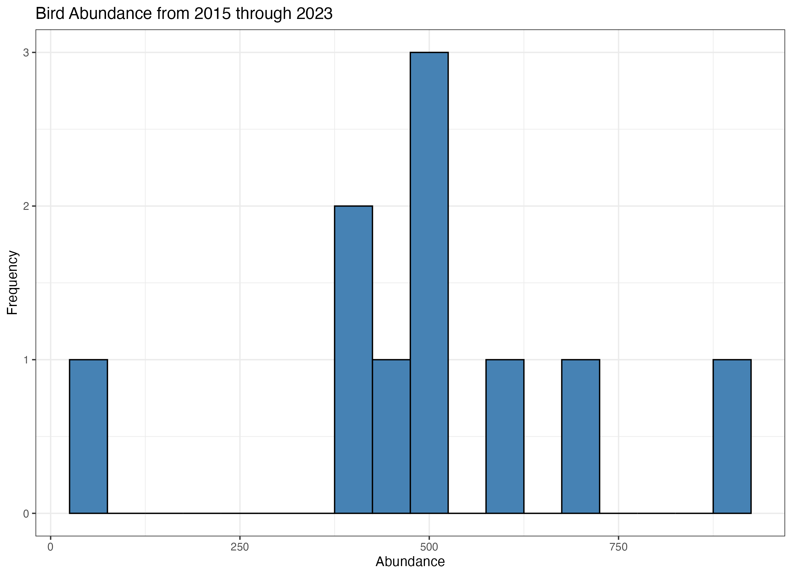
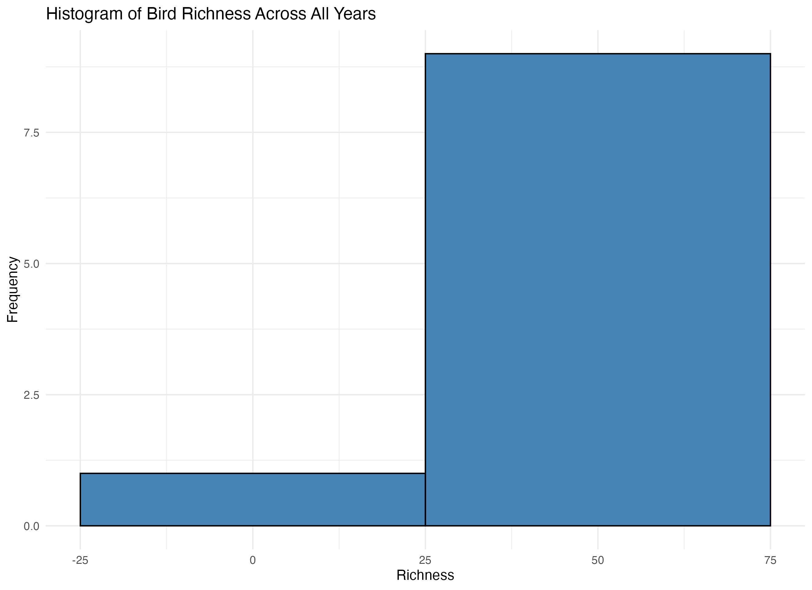
create_histograms(stats)
Results
Stats
| File Name | Abundance | Richness | Year |
| NEON.D01.BART.DP1.10003.001.brd_countdata.2015-06.basic.20241118T065914Z.csv | 459 | 40 | 2015 |
| NEON.D01.BART.DP1.10003.001.brd_countdata.2016-06.basic.20241118T142515Z.csv | 696 | 39 | 2016 |
| NEON.D01.BART.DP1.10003.001.brd_countdata.2017-06.basic.20241118T043125Z.csv | 411 | 35 | 2017 |
NEON.D01.BART.DP1.10003.001.brd_countdata.2018-06.basic.20241118T105926Z.csv |
515 | 37 | 2018 |
| NEON.D01.BART.DP1.10003.001.brd_countdata.2019-06.basic.20241118T064156Z.csv | 410 | 44 | 2019 |
| NEON.D01.BART.DP1.10003.001.brd_countdata.2020-06.basic.20241118T184512Z.csv | 489 | 46 | 2020 |
| NEON.D01.BART.DP1.10003.001.brd_countdata.2020-07.basic.20241118T010504Z.csv | 54 | 18 | 2020 |
| NEON.D01.BART.DP1.10003.001.brd_countdata.2021-06.basic.20241118T105538Z.csv | 920 | 50 | 2021 |
| NEON.D01.BART.DP1.10003.001.brd_countdata.2022-06.basic.20241118T033934Z.csv | 592 | 39 | 2022 |
| NEON.D01.BART.DP1.10003.001.brd_countdata.2023-06.basic.20241118T091043Z.csv | 523 | 42 | 2023 |
Regression Summary
| coef_abundance | intercept | r_squared | p_value_abundance | n_obs |
| 0.03137201 | 23.09753 | 0.6506631 | 0.004808103 | 10 |
Histograms